IS-LM and MMT
The core issue at the heart of debates between the heterodox Modern Monetary Theory (MMT) approach and more mainstream macroeconomics is how the financial economy and the real economy interact. As a consequence we see Keynesians of various hues attempting to illustrate their response to MMT with the standard orthodox Keynesian IS-LM model of the economy, which attempts to illustrate this interaction graphically
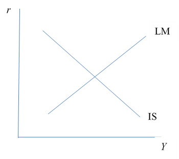
The IS-LM model, as elaborated by various economists after Keynes, consists of upward and downward sloping curves in income (Y) and interest (r) space. (See Figure 1) The downward-sloping IS curve illustrates the inverse relationship between the cost of physical capital (summarised by r) and GDP (Y) where investment is assumed to be the major variable in the latter. The upward-sloping LM curve is a somewhat more complex concept but essentially proposes that given a fixed supply of money, a higher Y leads to a higher interest rate on bank deposits. This interest rate is assumed to feed through to the price demanded for financial capital in such a way that it can be considered as variable r for the purposes of the model.[1] The model is thus somewhat vague in what r is really standing for. Further criticism is that a fixed supply of money is an unrealistic concept; the quantity of money supplied in a modern monetary economy being endogenous to its demand. It is also pointed out that the model mixes up stocks (of money) and flows (of income). Despite these criticisms, the IS-LM structure has been used to characterise MMT ideas in terms of the slopes of the two curves – in its extreme a vertical IS curve (implying investment as independent from any rate of interest) and a horizontal LM curve (implying a technically unlimited supply of money).
A Matching Flows Approach
A better way of approaching the real/money interaction might be to work from the viewpoint of two linked flows – that of money and that of its exchange counterparts. We start off with the economy in a steady state, with constant flows of money on one side and of real goods and services and speculative assets on the other. (See Figure 2) There is no distinction between consumer goods and services and productive capital goods in this model, since this is regarded as an arbitrary distinction between goods that have a spectrum of durability and of the timing of flows of utility and/or monetary return. What we will distinguish are goods purchased for use, and those (speculative assets) purchased for resale at (expected) higher prices.[2]
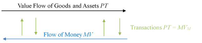
In our steady state the quantity equation holds:
MVM = PT = PZTZ+ PFTF , (1)
where PZ and PF are price indices of real goods and speculative assets respectively, and TZ and TF the numbers of transactions involving those. Total cash and bank deposits are represented by M. VM is the money velocity that would be calculated directly from this quantity equation if TZ and TF could be observed. If money flow MVM and total transactions T are constant this implies a constant P – the absence of inflation.
While MVM represents the aggregate flow of money, I argue that this is not the flow that actually adjusts to match the flow of goods and assets, and therefore is a misleading focus for determining the impact of changes in M. I introduce the concept of the effective flow of money by which I mean that part of the total money stock that is in continuous use for transactions. This is analogous to that part of an eddying stream that is in continuous directional motion. In terms of an economy that primarily uses deposit money, the effective flow is given by XVX where X = M – B and B is the monthly average minimum (positive) balance across all accounts.[3] (See Figure 3) Setting XVX = PT allows us to determine VX as a velocity specific to this flow. The effective flow of money is not directly observable in a deposit banking system without access to data at the level of individual deposits. As a consequence we cannot easily distinguish between the effective flow taking the form of the bulk of the measured quantity of money being turned over slowly (few or no ‘eddies’), and it being a smaller amount turned over more quickly (many eddies), but these different scenarios have different implications for impacts on economic activity. The relevant flow of money is XVX, but the velocity that would be calculated from the quantity equation would be VM which may well have no bearing on activity, because where B > 0, VX > VM.
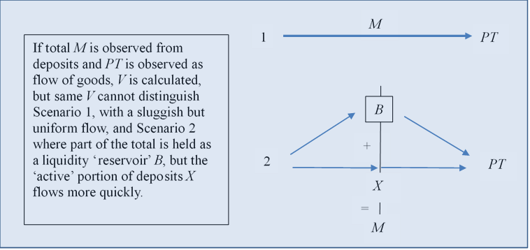
If the bulk of money gets turned over in a particular period, implying that minimum balances are close to zero such that X?M, it is difficult to see how this flow can be increased by much in the era of ubiquitous cash dispensers, contactless payments and FastPay deposit transfers. In this case a higher level of monetary exchange that demands a greater flow of money will require a greater quantity of money (M). If on the other hand most deposits remain significantly in credit (that is, they have an average minimum balances significantly greater than zero so that X < M), then there are inactive quantities of money which can be mobilised to increase the effective flow of money (XVX) without needing to inject additional quantities. Since this implies a matching increase in PT, without an increase in M we would calculate an increase in total velocity VM but this could mislead us as to what is actually taking place. Instead of a potentially long-term increase in money velocity we would have a short-term boost to effective flow, which without further money injection has limited sustainability. Reasons for minimum balances B to change could include changes in uncertainty, anticipated changes in the price level, the ‘rate of return’ (welfare and financial) on goods and financial assets, and the interest rates on deposits (if any, and depending on how they are calculated).
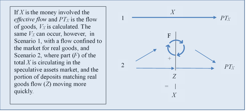
A further issue is that the retail price index is determined by PZ = ZVz/TZ where Z is the money used in that part of the effective flow of money circulating in the market for real consumption goods so that a pure increase in speculative asset transactions has no impact on this. In this case the relevant money velocity is now not the calculated VX from above, but the value VZ. If F is the quantity of money circulating in the market for financial assets then Z = X – F,or expanded, Z = M – B – F. (See Figure 4)
In summary, even if monetary exchange technology is thought to be pretty much stable, it is difficult to directly link changes in M to changes in the price level, since this is also mediated by changes in B, and by transfers between real goods and financial asset transactions. If an increase in production is planned, even if widespread, there is no direct way to link this with the mobilisation of ‘inactive’ deposits since these are not necessarily simply waiting for the right interest rate for them to be mobilised. If monetary and real goods flows are matched according to the quantity equation ZVz = PZTZ, minimum balances remain constant (are not mobilised) and the asset circulation stable, then to market additional goods may require an additional money flow – new money must be created to allow the purchase of required inputs on the basis of the future sale of outputs. In the private sector this requires that the anticipated monetary profit from the new production exceeds the cost of raising the new money by bank lending. In the public sector this implies a government calculation that the net welfare value of the new production is greater than the welfare cost of spending new money into circulation. (The matching of new private and public sector activity with the money required for the additional goods to enter the monetary economy is somewhat equivalent to movements along the IS and LM curves to arrive at ‘equilibrium’ values for Y and r. What is different is that there is in reality no need for an equilibrating mechanism – the new money is issued as part of the process of new production and cannot, in a monetary economy, be divorced from it.)
The Source and Consequences of New Money
What is the cost of raising new money? New money issue has a cost by being an institutional guarantee of an obligation. For a bank loan this involves monitoring costs, reserve costs and repayment risks for the loans issued. For the government the costs are those of imposing and collecting any additional taxes required to ensure the acceptance and to maintain the value of its money – these include the economic and political ‘distortions’ that may result from these new taxes (and vice versa, any positive benefit from taxation in term of the discouraging of costly behaviours should be deducted from the cost of issue).
‘Unbalanced’ Money Flow
If balancing revenue (in sales or as taxes) proves temporarily difficult (or overly costly) to obtain subsequent to the issue of new money, there are ‘smoothing’ mechanisms available. For private firms, bonds or equity can be issued to obtain funding to repay loans due. For the government, bonds can also be issued, but since the government has no higher authority it is obligated to, it can simply operate with a persistent shortfall in tax obligations. This is usually described as having ‘monetised’ debt and is generally frowned upon.[4] We could however reinterpret it as analogous to private firm’s equity. The money held in excess of tax and bond obligations represents a long-term claim on the government that does not entitle the holder to dividends, but may represent welfare-enhancing government activity, in which the holder may as a minimum ‘feel’ the benefit through solidarity with his or her fellow citizens.
In the same way that excessive equity issue by firms dilutes the value of the ownership in the firm that it represents, excessive monetisation of debt may dilute the value of claims on the government – with potential inflationary consequences. This depends in part on what citizens are able to and wish to do with this additional money. If the increased flow resulting from money issue is matched by an increased flow of goods from the private sector in response to a costless increase in liquidity – implying increased use of existing or easily-expanded facilities, or results in a net increase in the holding of minimum balances, then no inflationary pressure arises.[5] Another variable that impacts on the result of debt ‘monetisation’ is the extent to which any new government money enters the flow, not of real goods, but of financial assets. This may result in the increase in prices of financial assets (an increase in PF), which would not usually be considered as contributing to inflation. The nature of financial assets, however, is such that they can be created on the basis of future expectations alone, with an accompanying increase in TF, so that asset price rises need not necessarily occur. In summary, the monetisation of government debt need not necessarily lead to an increase in the price level for retail goods, and to the extent that it does the magnitude of the effect will be difficult to predict. Even if a retail price increase does occur, anything other than a one-off increase in the price level requires an amplification mechanism that links a general price rise to a general wage rise, followed by feedback to a new price rise. Significant structural changes in the labour market make this less likely to occur than it has been observed to do in the past.
Interest Rate Setting
If we see the aim of macroeconomic management being primarily to match real and financial flows in such a way as to enable physical resources to be fully utilised and allow real shocks to be accommodated without harmful price level fluctuations, then what is the role of the government in setting a base rate of interest for the private sector to access new money? If the private sector can be expected to match these flows according to its own efficiency criteria, the important issue appears to be to adjust for any externalities. If the cost of raising new money to match a new flow of goods involves the use of the central bank and government’s financial and payment infrastructure (in facilitating the free flow of reserves between banks, providing an interface for banks to access reserves as needed and regulatory oversight) then efficiency demands that the costs of maintaining this are internalised to the private banks. In other words the efficient interest rate on loans of reserves from the central bank (the base rate) is such that the central bank (on average) covers its costs.
As long as private firms and banks calculate the potential sales of new output reasonably accurately (and their own incentives are in line with this) then their ability to create new money should not be inflationary and the reasoning above on the base rate follows. There are two main reasons for thinking that this line of reasoning may not be the whole story, and these result from co-ordination issues between individual private banks. There is a negative co-ordination problem in that individual banks may not know in advance whether new production they are funding is entering an exclusive market. If it is not, then revenue predictions and thus loan repayment ability may be less than predicted. Loan defaults are a problem for banks alone as long as their equity buffers are not breached. An alternative strategy for a firm that anticipates a smaller market for its output than initially expected is to raise its prices. Under certain conditions, particularly where prices and wages are already rising for other reasons, it may get away with this. If this behaviour becomes widespread then inflation may result. The second issue is a positive co-ordination problem, where banks anticipate each other providing the finance to bid up the prices of speculative assets – so that any lending can be recouped with each successive sale. What we have here is bubble formation. In both cases raising the reserve costs for banks through base rate rises may act, at least in theory, as a disincentive to welfare-inefficient lending and new money creation.[6] While a cost price base rate is the first-best solution under ideal bank behaviour, when this behaviour moves away from the ideal an adjusted rate may be an improving intervention. On the other hand, there may be more targeted interventions against bank and firm behaviour that are more efficient than setting an ‘inefficient’ bank rate. The base rate may not only impact on new money creation for the target sector, but also in unintended and unpredictable ways on minimum balances and other market sectors. The use of the speculative asset market as a mechanism for determining real goods allocations for certain groups (especially the retired) makes the latter particularly problematic here. So MMT’s set of fiscally-based interventions – particularly where their operation is intended to be automatic – are well worth consideration. Fiscal interventions can be more specifically tailored to particular flow problems arising in individual sectors.
The Job Guarantee as an Automatic Fiscal Intervention
The essence of the job guarantee (JG) scheme, which is regarded by many MMT adherents as the foremost and most essential of fiscal interventions, is that it is a highly targeted form of economic stimulus with an inbuilt stabilising mechanism, and so to some extent avoids the criticisms of otherwise sympathetic commentators of the political economy problems of the implementation and timing of fiscal interventions.[7] JG wages enter the monetary flow matching real goods exchanges specifically. The proposed stabilisation mechanism arises because the guaranteed jobs are at or around the minimum wage level, with the result that any increase in economic activity would be expected to increase the level of private-sector employment, thus decreasing the number of those receiving the JG and dialling down its macroeconomic impact. Moreover, the JG scheme is contrasted favourably by its advocates with a basic income scheme of welfare in that it is more supportive of the stability of a monetary economy, which we could interpret as its being superior in maintaining the stable matching of the monetary flow and the flow of real goods and services.
Conclusion
Modern Monetary Theory and its policy proposals are both supported and undermined by the uncertainty surrounding differential and potentially variable monetary velocities. Supported in that the relationship between government deficits and the consequent flow of government money into circulation to price changes and inflation is not subject to hard and fast rules that mandate ‘balanced budgets’; undermined in that the lack of any such rules make any fiscal intervention risky. The same uncertainty considerations apply to the desire to de-emphasise the role of stabilisation policy through interest rates. Moreover, as Palley (op cit) points out, tax rises are inevitably subject to significant political pressure, and any proposed policy framework change induces expectations whose consequences may be immediately felt – whether or not those expectations are rational. These problems with macroeconomic policy, relying as it does on predictions of aggregate effects from the actions of millions of individuals, should point us in the direction of immediately tackling real human and social needs with the real resources at our disposal and of mitigating directly the gross inequality of power over those resources.
[1] In fact empirical evidence suggests that aggregate business investment is difficult to clearly correlate to rates of interest. For a concise recent overview see Hambur J. and La Cava G., 2018, Do Interest Rates Affect Business Investment? Evidence from Australian Company-level Data Research, Discussion Paper 2018-05 Economic Research Department Reserve Bank of Australia.
[2] In reality these are not mutually exclusive categories – property for example falling into both – so to operationalise this some weighting would be required.
[3] The choice of monthly minimum balances is somewhat arbitrary and based on the most common income interval. It might turn out on empirical investigation that some other interval might correlate better with the variables of interest, but this is work for the future.
[4] Or in some monetary jurisdictions – such as the US – specifically disallowed by current legislation.
[5] The former indicates that the private sector could have taken on debt to pay workers for new output that would have been consumed with the new money, but they did not do so – which is form of collective action problem that the government’s addition to the money stock has rectified. If the new level of productive activity is maintained with a consistently higher effective flow XVX, there may be no need for the imposition of new taxes at any point.
[6] Conversely, revenue and loan repayment might be consistently underpredicted, in which case a lower level of interest rate might be welfare-enhancing depending on the sensitivity of bank lending to the base rate.
[7] See eg.: Palley T. 2019, What’s Wrong With Modern Monetary Theory (MMT): A Critical Primer, Forum for Macroeconomics and Macroeconomic Policies Working Paper 44